StrainDesign

A COBRApy^[1]-based package for computational design of metabolic networks

The comprehensive StrainDesign package for MILP-based strain design computation with the COBRApy toolbox supports MCS, MCS with nested optimization, OptKnock ^[2], RobustKnock ^[3] and OptCouple ^[4], GPR-rule integration, gene and reaction knockouts and additions as well as regulatory interventions. The automatic lossless network and GPR compression allows strain design computations from genome-scale metabolic networks. Supported solvers are GLPK (available from COBRApy), CPLEX, Gurobi and SCIP ^[5].

Installation instructions ...

Download Jupyter notebook examples ...

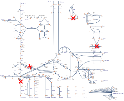
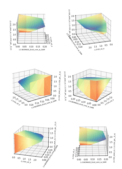
The default compression uses a pure Python sparse RREF implementation. A legacy Java-based compression via EFMTool ^[6] is optionally available (see Legacy Methods). Note that the Java backend (via JPype) is known to conflict with CPLEX’s native library when both are loaded in the same Python session. If you use CPLEX, we recommend the default Python compression backend.

Installation:

The StrainDesign package is available on pip and Anaconda. To install the latest release, run:

pip install straindesign

or

conda install -c cnapy straindesign

Developer Installation:

Download the repository and run

pip install -e .

in the main folder. Through the installation with -e, updates from a ‘git pull’ are at once available in your Python environment without the need for a reinstallation.

Apple Silicon (ARM64) note:

On macOS with Apple Silicon (M1/M2/M3), the default GLPK solver (shipped with COBRApy) may produce inaccurate results for larger metabolic models due to numerical precision differences on the ARM64 architecture. If you encounter unexpected infeasibility or incorrect flux values, we recommend installing an alternative solver:

• Gurobi (free academic license): pip install gurobipy

• SCIP (open source): pip install pyscipopt

Then specify the solver explicitly when calling StrainDesign functions, e.g. sd_setup = {..., 'solver': 'gurobi'} or sd_setup = {..., 'solver': 'scip'}. For standalone analysis functions: fba(model, solver='gurobi') or fva(model, solver='scip').

Examples:

Computation examples are provided in the different chapters of this documentation. The original Jupyer notebook files are located in the StrainDesign package at docs/source/examples.

How to cite:

Schneider P., Bekiaris P. S., von Kamp A., Klamt S. - StrainDesign: a comprehensive Python package for computational design of metabolic networks. Bioinformatics, btac632 (2022)

Contents:

• Solvers
  • 3rd party solver installation
    • CPLEX
    • Gurobi
    • SCIP
  • Solver selection
• Network Analysis
  • Flux optimization (FBA/pFBA)
    • Parsimonious FBA (pFBA)
  • Flux variability analysis (FVA)
  • Gene knockout simulation
  • Yield optimization
    • Mathematical background
• Plotting the flux space
  • Production Envelopes
  • Yield Spaces
  • Mixed Plots
  • 3D plots
    • Interactive and animated 3D plots
• Computational strain design: Growth-coupled production (GCP)
  • pGCP: potentially growth-coupled production
  • wGCP: weakly growth-coupled production
  • dGCP: directionally growth-coupled production
  • SUCP: substrate-uptake-coupled production
• Minimal Cut Sets (MCS)
  • Prerequisites
    • 1) Add and verify production pathway
  • Example 1: Strain designs with a minimum product (1,4-butanediol) yield (SUCP strain design)
  • Example 2: Enforce product (1,4-BDO) synthesis at all growth states (dGCP strain design)
  • Example 3: Suppress flux states that are optimal with respect to a pre-defined objective function (wGCP strain design)
  • Example 4: Protect flux states that are optimal with respect to a pre-defined objective function (pGCP strain design)
  • Example 5: All single gene knockouts that prohibit growth (synthetic lethals).
  • Example 6: Genome-scale strain designs with a minimum product (1,4-butanediol) yield (SUCP strain design)
  • Example 7: Suppress flux states in a toy network
  • Example 8: Suppress and protect flux states in a toy network
  • Theoretical background
• Multi-level strain optimization approaches
  • OptKnock
    • Example 9: OptKnock strain design
    • Example 10: OptKnock strain design with a tilted objective function
    • Example 11: Genome-scale OptKnock strain design
  • RobustKnock
    • Example 12: RobustKnock strain design
  • OptCouple
    • Example 13: OptCouple strain design
  • Combining nested optimization strain design with MCS
    • Example 14: Combining OptKnock with a tilted objective function and the MCS approach
• Standalone network compression
  • Standalone GPR-integraton
    • Gene perturbation studies
• CNApy interface
• StrainDesign API
  • straindesign
    • Submodules
      • straindesign.compression
      • straindesign.compute_strain_designs
      • straindesign.cplex_interface
      • straindesign.efmtool_cmp_interface
      • straindesign.glpk_interface
      • straindesign.gurobi_interface
      • straindesign.indicatorConstraints
      • straindesign.lptools
      • straindesign.names
      • straindesign.networktools
      • straindesign.parse_constr
      • straindesign.pool
      • straindesign.scip_interface
      • straindesign.solver_interface
      • straindesign.speedy_fva
      • straindesign.strainDesignMILP
      • straindesign.strainDesignModule
      • straindesign.strainDesignProblem
      • straindesign.strainDesignSolutions
    • Package Contents
      • DisableLogger
• Legacy Methods
  • Java-based EFMTool compression (compression_backend='efmtool_rref')
  • JAVA_HOME path
• StrainDesign Developer’s Guide
  • How to read this guide
  • Chapters at a glance
  • Repository structure
  • 1. Orientation & the strain-design problem
    • 1.1 The metabolic model
    • 1.2 Desired vs. undesired flux regions
    • 1.3 SUPPRESS and PROTECT: precise semantics
    • 1.4 The bilevel variants (conceptual only)
    • 1.5 Interventions, costs, the binary vector z, and “minimal”
    • 1.6 The end-to-end pipeline at a glance
    • 1.7 How the package is invoked
    • 1.8 Notation reference
  • 2. The constraint-based foundation
    • 2.1 Mass balance and the steady-state assumption
      • 2.1.1 From dynamic mass balance to S·v = 0
      • 2.1.2 Dimensions, rank, and what the solution set is
    • 2.2 Bounds, reversibility, and the flux polytope
      • 2.2.1 Bounds encode direction and capacity
      • 2.2.2 The steady-state flux set is a polyhedron (cone / polytope)
    • 2.3 Exchange / boundary reactions
    • 2.4 FBA and FVA as linear programs — and how the code builds them
      • 2.4.1 FBA: one LP
      • 2.4.2 FVA: 2n LPs
    • 2.5 Enough polyhedral theory for Ch 6
      • 2.5.1 Faces, vertices, rays, recession cone
      • 2.5.2 Why an objective goes unbounded → the dual is infeasible
      • 2.5.3 Why an infeasible target region yields a Farkas certificate
    • 2.6 The standard form and build_primal_from_cbm
      • 2.6.1 Mapping a cobra model into the standard form
      • 2.6.2 The bookkeeping matrices (z_map_*)
  • 3. Network compression
    • 3.1 Why compress at all
    • 3.2 The exact integer/rational nullspace engine
      • 3.2.1 Why never float
      • 3.2.2 RationalMatrix and exact storage
      • 3.2.3 Fraction-free integer RREF: _rref_integer_sparse
      • 3.2.4 Reading off the kernel: _nullspace_sparse
      • 3.2.5 The big-integer path — when subdeterminants exceed int64
    • 3.3 The compression working state and the single-kernel pass
    • 3.4 Coupled / flux-coupled merge
      • 3.4.1 The math: why coupled reactions share a kernel pattern
      • 3.4.2 Detection: _find_coupled_groups
      • 3.4.3 The merge (COLUMN reduction): _combine_coupled
      • 3.4.4 Bound intersection of a coupled group
    • 3.5 Conservation-relation removal (ROW-rank reduction)
    • 3.6 Blocked and zero-flux removal
    • 3.7 The alternating fixpoint
    • 3.8 Parallel merge
    • 3.9 GPR propagation through compression
    • 3.10 The compression map cmp_mapReac and back-expansion
    • 3.11 The legacy efmtool (Java) backend
      • 3.11.1 What efmtool is and how straindesign reaches it
      • 3.11.2 Data marshalling: cobra model → Java → cobra model
      • 3.11.3 Why it is legacy
      • 3.11.4 Behavioral differences to be aware of
  • 4. GPR integration
    • 4.1 Why encode gene logic as flux structure at all
    • 4.2 extend_model_gpr: turning a rule into pseudo-metabolites and pseudoreactions
      • The gene gadget (leaf / ast.Name)
      • The and gadget (ast.And)
      • The or gadget (ast.Or)
      • Attaching the rule to the guarded reaction
      • Worked example: (g1 and g2) or g3
    • 4.3 Why the original flux space is unchanged (the correctness invariant)
    • 4.4 Reversible-reaction split and the reac_map remap
    • 4.5 reduce_gpr: pruning before extension
    • 4.6 The two-compression-pass boundary and why regulatory genes are exempt from pass #1
    • 4.7 Name truncation (sha256), Gurobi/GLPK only
  • 5. FVA in preprocessing
    • 5.1 The essentiality test — geometry of min(abs(range)) > 1e-10 and prod(sign(range)) > 0
    • 5.2 FVA #1 — essential reactions in PROTECT/desired modules (pre-GPR)
    • 5.3 FVA #2 — bound_blocked_or_irrevers_fva: relaxing non-binding bounds
      • Why relaxing a provably non-binding bound to ±∞ shrinks and conditions the MILP
    • 5.4 FVA #3 — knockable-scoped essentials and size-1 MCS extraction
    • 5.5 The speedy_fva acceleration engine
      • Bookkeeping and the “resolved” mask
      • Phase 1 — global scan LPs
      • Phase 2 — individual LPs for the residual
      • Internal compression (compress) and result expansion
      • Contrast with fva_legacy
    • 5.6 Why FVA #2 is the ~117 s genome-scale bottleneck
  • 6. Dualization (the mathematical core)
    • 6.1 Why dualize at all
    • 6.2 LP duality refresher, in the exact standard form the code uses
      • 6.2.1 Primal standard form
      • 6.2.2 Weak duality, strong duality, complementary slackness
      • 6.2.3 LP_dualize line by line
      • 6.2.4 What LP_dualize does and does not guarantee
    • 6.3 Farkas’ lemma and the SUPPRESS infeasibility certificate
      • 6.3.1 The lemma
      • 6.3.2 farkas_dualize
      • 6.3.3 Why the certificate is unbounded by nature, and the normalization row
      • 6.3.4 The b^T y ≠ 0 caveat
    • 6.4 Strong-duality encoding of bilevel problems
      • 6.4.1 The coupling row
      • 6.4.2 Exact vs relaxed inner optimality
      • 6.4.3 Optional outer objective on PROTECT/SUPPRESS
    • 6.5 One dualization, reused across every module type
      • 6.5.1 Inner-objective PROTECT / SUPPRESS (strainDesignProblem.py)
      • 6.5.2 OptKnock — bilevel max-min (strainDesignProblem.py)
      • 6.5.3 RobustKnock — three levels, two nested dualizations (strainDesignProblem.py)
      • 6.5.4 OptCouple — growth-coupling distance (strainDesignProblem.py)
      • 6.5.5 DoubleOpt — two parallel strong-duality links (strainDesignProblem.py)
      • 6.5.6 The unifying picture
    • 6.6 Boundary with Chapter 7
  • 7. MILP construction & the z-linking
    • 7.1 Notation and the shape of the master problem
      • The three z-maps
    • 7.2 SDProblem.__init__ — the seed rows, num_z, and the M switch
      • The three fixed seed rows
      • self.M — the master indicator/big-M switch
    • 7.3 addModule — block-diagonal assembly
      • Why block-diagonal for the continuous part
      • Why the z-columns are shared
    • 7.4 prevent_boundary_knockouts — why nonzero-sign bounds must be moved
      • The KO encoding and the failure
      • The transformation
    • 7.5 link_z — the heart of the chapter
      • Step 1: knockable equalities → ± inequality pairs
      • Step 2: variable-KOs → inequality rows
      • Step 3: the per-constraint bounding LP
      • Step 4: the fork at the M value
      • Steps 5–6: indicators and cleanup
    • 7.6 Indicator constraints (indicatorConstraints.py)
    • 7.7 Why indicators give a tighter LP relaxation than big-M
    • 7.8 The emergent SUPPRESS→indicator / PROTECT→big-M split
    • 7.9 Final consolidation and the binary block
  • 8. Solving & enumeration
    • 8.1 The objective is both a vector and a constraint row
    • 8.2 solveZ / solve: what one solver call returns
    • 8.3 The three approaches, their objective setups, and why
      • 8.3.1 ANY — compute (strainDesignMILP.py): feasibility-first, then subspace minimization
      • 8.3.2 BEST — compute_optimal (strainDesignMILP.py): global optimum, then fix and iterate
      • 8.3.3 POPULATE — enumerate (strainDesignMILP.py): native solution pool per cost level
    • 8.4 The iterative loop and integer cuts (the minimal-and-distinct guarantee)
      • 8.4.1 The superset-excluding cut — add_exclusion_constraints (:162-181)
      • 8.4.2 The exact-pattern cut — add_exclusion_constraints_ineq (:183-198)
    • 8.5 verify_sd: re-checking validity in the true continuous subsystem
    • 8.6 Solver parameters and determinism
      • 8.6.1 No MIP optimality gap is set — the 1e-4 consequence
      • 8.6.2 The solution-pool parameters are inert for single solve
      • 8.6.3 Seed → branch-and-bound tree shape → why speed needs a distribution
    • 8.7 Verified performance: the phase timeline and CPLEX vs Gurobi
    • 8.8 How SCIP and GLPK differ
  • 9. Decompression & solution semantics
    • 9.1 Why decompression is needed, and the shape of the compression map
    • 9.2 The math of reverse expansion (expand_sd)
      • Case KO of a parallel group (val < 0, par_reac_cmp True)
      • Case KO of a coupled group (val < 0, par_reac_cmp False)
      • Case KI of a group (val > 0)
      • Case KI not introduced (val == 0)
      • A worked micro‑example
    • 9.3 Size‑1 MCS re‑injection
    • 9.4 filter_sd_maxcost: why a post‑expansion cost re‑check is mandatory
      • The lazy‑expansion path (estimated count > 100 000)
    • 9.5 KI/KO value encoding and the strip semantics
    • 9.6 Gene‑level vs reaction‑level translation (_translate_genes_to_reactions)
  • 10. Known issues, gotchas & failure modes
    • 10.1 Issue #43 (OPEN) — gene-level designs with no reaction-level effect
      • Mechanism 1 — reduce_gpr pops protected/essential genes by id only
      • Mechanism 2 — _translate_genes_to_reactions evaluates the GPR only over solution-present genes
      • The id-vs-name fragility, end to end
    • 10.2 Issue #38 (OPEN) — superset/subset (non-minimal) solutions
      • The leading explanation: a reporting artifact from value-0 KI markers
      • The genuine residual: numerical-boundary non-minimality
    • 10.3 Issue #44 (CLOSED 2026-06-23) — PROTECT violated under gene_kos, as a cautionary tale
    • 10.4 Gotcha (a) — compute_strain_designs mutates the caller’s reg_cost/module dicts in place
    • 10.5 Gotcha (b) — Gurobi/GLPK-only name truncation (sha256; CPLEX exempt)
    • 10.6 Gotcha (c) — solver numeric-status robustness (Gurobi 12 NUMERIC; CPLEX 5/6 unscaled-infeasibilities)
    • 10.7 Other footguns
  • 11. Performance, benchmarking & roadmap
    • 11.1 The verified bottleneck profile
      • 11.1.1 Where the seconds go (canonical iML1515, CPLEX)
      • 11.1.2 The CPLEX-vs-Gurobi ≈4.4× gap and its true causes
    • 11.2 The performance levers
      • 11.2.1 Compression depth = rank / z-count reduction (the structural lever)
      • 11.2.2 MILP formulation & conditioning
      • 11.2.3 Skip hopeless big-M / dual work
      • 11.2.4 The Farkas-dual pre-bounding problem (the known hard lever)
      • 11.2.5 The whole-model preprocessing FVA
      • 11.2.6 Enumeration & pooling strategy
    • 11.3 Benchmarking discipline
    • 11.4 Roadmap & directions
  • 12. Model surgery & constraint parsing
    • 12.1 remove_ext_mets — deleting the boundary layer before compression
    • 12.2 parse_constr.py — strings into A·x {≤,=,≥} b
      • 12.2.1 The scanner: linexpr2dict / linexpr2mat
      • 12.2.2 The (in)equality splitters: lineq2mat, lineq2list
      • 12.2.3 The dispatcher: parse_constraints
    • 12.3 extend_model_regulatory — a bound as an intervention
      • 12.3.1 The encoding math
      • 12.3.2 Name generation and the in-place dict mutation (footgun)
      • 12.3.3 Reaction-based (immediate) vs. gene-based (deferred)
    • 12.4 gene_kos_to_constraints — a gene KO set as flux constraints
    • 12.5 Module & cost compression — keeping references consistent with a moving index
      • 12.5.1 The remapping math
      • 12.5.2 Cost remapping and the parallel/coupled asymmetry
    • 12.6 Ordering, and why it is load-bearing
  • 13. The object model & result API
    • 13.1 SDModule — the problem-specification object
      • 13.1.1 What it is: a validated dict subclass
      • 13.1.2 The six module types
      • 13.1.3 Per-type validation, step by step
      • 13.1.4 Construction examples
    • 13.2 SDSolutions — the result object
      • 13.2.1 What a “design” is: the intervention dict
      • 13.2.2 Internal storage
      • 13.2.3 The public accessor contract
      • 13.2.4 Lazy expansion and representatives (PR #40)
      • 13.2.5 Save / load and model embedding
    • 13.3 The sd_setup object — one bundle, two roles
      • 13.3.1 The key set
      • 13.3.2 Role 1 — sd_setup as INPUT
      • 13.3.3 Role 2 — sd_setup as OUTPUT / reproducibility record
      • 13.3.4 Downstream uses — why a self-contained setup pays off
    • 13.4 The preprocessed-dump workflow
      • 13.4.1 Dumping: dump_preprocessed
      • 13.4.2 Replaying: compute_strain_designs_from_preprocessed
      • 13.4.3 The developer workflow
  • 14. The solver-interface layer (MILP_LP + backends)
    • 14.1 Why an abstraction layer exists
    • 14.2 The canonical problem and the MILP_LP constructor
    • 14.3 The three solve entry points and result normalization
    • 14.4 Indicator constraints vs big-M, per backend
    • 14.5 Status-code translation to the canonical vocabulary
    • 14.6 Parameters: seed, threads, tolerances, time limit, working memory
    • 14.7 The solution pool: native (CPLEX, Gurobi) vs emulated (SCIP, GLPK)
    • 14.8 Numeric-status robustness
    • 14.9 Where the CPLEX-vs-Gurobi performance story physically lives
  • 15. Analysis & exploration API
    • 15.1 fba — flux balance analysis and its parsimonious variants
      • Contract
      • Unbounded-objective repair
      • Parsimonious FBA (pfba)
      • The compressed-flux hook
    • 15.2 fva — flux variability analysis as a public tool
    • 15.3 yopt — yield optimization by linear-fractional programming
      • What and why
      • The transform
      • The sign of the denominator — den_sign
    • 15.4 plot_flux_space — production envelopes, yield space, and 3D projections
      • What it visualizes
      • Axis grammar
      • The mathematics of a production envelope
    • 15.5 Compressed-analysis tools (PR #56)
      • expand_fluxes — lifting a flux vector
      • slim_fba_via_cmp — objective-only FBA on the compressed model
      • Compressed plot_flux_space
    • 15.6 Where these fit the developer’s workflow
  • 16. Testing & contributing

References:

[1] Ebrahim, A., Lerman, J.A., Palsson, B.O. et al. - COBRApy: COnstraints-Based Reconstruction and Analysis for Python. BMC Syst Biol 7, 74 (2013)

[2] Burgard, A. P., Pharkya, P., & Maranas, C. D. - Optknock: a bilevel programming framework for identifying gene knockout strategies for microbial strain optimization. Biotechnology and bioengineering, 84(6), 647–657 (2003)

[3] Tepper N., Shlomi T. - Predicting metabolic engineering knockout strategies for chemical production: accounting for competing pathways, Bioinformatics. Volume 26, Issue 4, Pages 536–543 (2010)

[4] Jensen K., Broeken V., Lærke Hansen A.S., et al. - OptCouple: Joint simulation of gene knockouts, insertions and medium modifications for prediction of growth-coupled strain designs. Metabolic Engineering Communications, Volume 8 (2019)

[5] Bestuzheva K., Besançon M., Chen W.K. et al. - The SCIP Optimization Suite 8.0. Available at Optimization Online and as ZIB-Report 21-41, (2021)

[6] Marco Terzer, Jörg Stelling, Large-scale computation of elementary flux modes with bit pattern trees, Bioinformatics, Volume 24, Issue 19, (2008), Pages 2229–2235,

Indices and tables

• Index

• Module Index

• Search Page